Fiddling with bytes to make satellite image basemaps, or alternatively, the story of how I blindly fumbled around publicly available data, numpy, and claude code. This is a, in a way, part 5 in the ‘(Mis)adventures in AI CLIs’ series. It is not titled as such though because this is more about my own naive python data pipelines mistakes and notes to avoid repeating them in the future than it is about claude code or codex.
Conclusions Advice upfront.
There are no magic recommendations here, just advice. Important context, the goal is to run a python, numpy, based application in Google Cloud Platform (GCP) Cloud Run as a scheduled task. The application simultaneously processes up to four 100 million element floating point numpy arrays–more detail below. Cloud Run is serverless mechanism for running containers. I do not have to configure VMs or a managed kubernetes cluster in return for working within a restrictive set of configurations. The main downside is the allowed CPU-memory combinations were poorly suited for my application’s initial code which would consume ~8GB of resident memory space while using only a single CPU thread.
Advice,
- Starting with the most obvious, arithmetic operations on an numpy array, hereafter ’ndarray’, yield new arrays. Each array consumes memory. Many operations on large ndarrays may consume a large amount of memory.
- Claude Code oft suggested explicitly dereferencing large ndarrys using
del. This was largely unhelpful and only had small impacts on total memory use. I suspect this was the case because the application is reasonably well factored with small methods resulting in intermediate or temporary ndarrays being quickly garbage collected. See screenshot.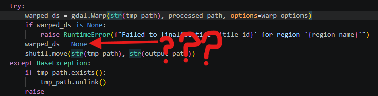
The
deldoes nothing, there are other issues here too discussed below - One-shot prompting either Sonnet or Opus models to perform a memory usage analysis was unhelpful. Both models focused on GDAL’s cache setting instead of multiple large ndarrays. The quality of analysis improved when given screenshots of resource utilization, but still failed to identify key issues.
- I had to guide with direction setting prompts to get useful changes out of Claude. For example, “Consider the total utilization of 8GB combined with when the application writes files to disk. Can you please specifically analyze the color enhancement function,
true_colorfor memory use and propose ways of reducing the size of the working set.` This should sound familiar to readers of prior posts; ultimately, I still needed to understand the application’s function in order to get the most of claude.
- I had to guide with direction setting prompts to get useful changes out of Claude. For example, “Consider the total utilization of 8GB combined with when the application writes files to disk. Can you please specifically analyze the color enhancement function,
- The change that made the biggest difference in memory was also the conceptually most simple. Just process less in parallel. The application streams data to process from a remote host already. In order to reduce memory I changed from loading all four ndarrays entirely memory to windowed processing of the arrays 2000 elements at a time.
- All the above said, if this was a prototype for a business I would have likely started with a virtual machine like the C4 or N4 high memory series and been able to run my unoptimized code immediately. My couple hour a week hobby project is not a business use case though and I want to optimize for learning, ease of clean up, and cost.
- Do not trust Claude Code to do smart optimizations. At least not without guidance so precise that it may make sense to make changes yourself. For example, I got results ranging from half-baked to non-functional from Claude after directing to optimize for running the software in a “serverless context like Google Cloud Run with a Google Cloud Storage output”.
- Make sure you or Claude are actually doing performance tests. In my particular use case lossless WebP compression proved superior to JPEG-XL compression.
So anyway what is the ‘application’?
I’ve been working on a small utility that generates a mosaic of Copernicus Sentinel land monitoring data. Specifically, the utility combines the red, green, and blue visible bands from the Sentinel-2 Quarterly Cloudless Mosaics. The general algorithm is,
- Start with a closed polygon defined using latitude and longitude points
- Get the list of Sentinel-2 Quarterly Cloudless Mosaic tiles that cover the defined region
- Use the red, green, and blue tile data to create color images
- There are several sub-steps here to enhance image contrast and saturation and to convert from floating point “digital numbers” to 24-bit color. This is also the origin of most of the application’s memory use.
- Mosaic each Sentinel 110km by 110km tile into a larger regional mosaic
- Use regional mosaics to generate tile pyramids for use in web maps
Sentinel-2 data, and similar level 2 data from the USGS Landsat program, is not immediately usable for map imagery. They contain georeferenced “digital numbers” based on the amount of reflected light within specific wavelengths. Confusingly the specific meaning of ‘digital number’ differs between the European and USGS programs despite use of the same phrase in similar contexts. This page has information about the data available from Sentinel.
Sentinel data is available as geotiffs, one band–or in our case, color wavelength–per file. Each file represents an approximately 110km by 110km square on the earth with a resolution of 10m per pixel.
Small aside about satellite imagery
We do not marvel enough at the imaging technology deployed by Airbus systems, Vantor, and others that captures high resolution satellite imagery used in Google Maps.
Sentinel’s 10m per pixel is reasonably good resolution and works well for my purposes. Vantor (formerly Maxar Technologies) proudly advertises their global 30cm per pixel resolution mosaics. Similarly, Airbus also advertises up to 30cm per pixel spatial resolution. That’s two orders of magnitude higher resolution than Sentinel-2, one of the best publicly and freely available data sources. For context, this is the difference between being able to count major throughways like highways vs. being able to count individual driveways with cars in them.
All this from an sensor package on a satellite ~430 miles or ~700km above the surface of Earth.
Issues and corrections in detail
How (not) to accumulate a large number of pixels
I, enabled by Claude, wrote some code that attempted to accumulate up to 85 separate Sentinel-2 mosaic tiles into a single file.
I thought it made sense to accumulate the data into a single file.
I thought ZSTD compression would be enough.
I thought that claude code generated reasonable gdal geotiff creation options..
These thoughts were incorrect. Let’s discuss the issue.
Each Sentinel-2 Quarterly Cloudless Mosaic ’tile’ is served as up to four separate downloaded files. Each file is a geotiff containing a single band of information. We are interested in three files containing red, blue, and green light reflectance values. Each file is uncompressed and is approximately 150MB. Blindly combining these would result a ~450MB file for each 110km by 110km square. 110km by 110km square tiles sound large, but I need 85 of these to cover just one of the areas I want to map. For reference, \(450 MB \times 85 \approx 38GB \); this is a decently large file.
Since the application processes data progressively by downloading from Sentinel it also progressively writes the output file. This requires care too. GDAL’s geotiff driver requires that the accumulator file exist ahead of time in its final resolution and pixel size in order progressively accumulate data. Ideally the file is created with GDAL’s “SPARSE_OK=TRUE” creation option so that nothing is written when opening a very large empty file. Not using this option ironically results in more data written to disk to indicate that the file starts with no data. Claude Code’s generated code missed this option. That being said, missing the option is relatively benign and results in a slower application startup.
Less benign though was Claude’s generated code missing the predictor configuration for ZSTD compression which resulted in a larger than optimal compressed file. Fixing these two issues improves startup time and reduces to final output size to less than 18GB from 38GB.
These fixes are irrelevant though because 18GB is also larger than the available (preview feature) ephemeral scratch space for Cloud Run. I could progressively write a large file like this from the cloud run function to a cloud storage mount but this might risk corruption to due network or other unanticipated connectivity failures.
The real fix is to change the application design to use a more common geospatial processing pattern. Each Sentinel-2 tile should be processed into a true color compressed tile. A GDAL virtual file can be defined over the set of tiles for downstream processing. Using VRT has some drawbacks, but they are not applicable to my particular use case of handling preprocessed cloudless Sentinel-2 mosaics.
After this fix, step #4 above changed from writing a single ‘regional mosaic’ file into writing each tile from step #3 to disk and then creating a GDAL VRT.
Making things smaller
JPEG-XL compresses rasters really well at the cost of time and is the newest raster codec generally supported by GDAL. I assumed that newest meant best. I was wrong. Again.
JPEG-XL with a high effort compression setting might be another approach to reducing the per-region mosaic file size in step #4 to under 10GB per file. Unfortunately, while JPEG-XL compresses raster images well, the high effort compression settings also take a long time–as in, several minutes per Sentinel-2 tile on my laptop and up to 30 minutes per tile in a 4 core GCP Cloud Run container.
Aside, I have read rumors that the reason JPEG-XL has not been adopted widely in browsers is due to the decoder’s relatively high CPU consumption.
I decided to test compression settings as part of one of several rounds of hand tuning. Lossless WebP turned out to compress nearly as well and in some cases better than JPEG-XL with an effort of 6. Lossless WebP is also faster by nearly a factor of four on Cloud Run. Go figure.
Resiliency
Claude Code generated both standard resiliency changes and some pretty useless changes. On the good side, adding HTTP request retries with exponential backoff was helpful when dealing with the Copernicus STAC API which is heavily rate limited.
On the useless side of things, Claude Code generated a write-then-copy scheme where outputs are written to a temporary file in /tmp and then copied to the final output. I understand the intuitive logic of this and why source material across the internet might suggest it, but the approach makes assumptions about the application’s operating environment that are not always true. In our case, the Google Cloud Storage FUSE drive includes caching and retries anyway that make this feature superfluous.
Much less helpfully, Claude Code generated non-pythonic code that failed to use python context handlers in multiple locations meaning that try-finally statements were need to clean up file handles. I fixed these manually.
On the topic of threading
GDAL has confusing threading options. Claude Code also got them mostly wrong. I got them wrong for a while too.
Things to note,
- GDAL_NUM_THREADS
- Number of python workers independently processing tiles
- Certain GDAL operation’s
mutlithreadoption, for example gdal.warp
Summarizing what I learned and where I ended up,
- Most of GDAL’s inner workings and algorithms are single-threaded for any given block of data. They are re-entrant and can used to process multiple different blocks of data in parallel.
- GDAL_NUM_THREADS broadly controls the threading used by underling compression and decoding algorithms in GDAL’s drivers. This usually defaults to ‘ALL_CPUS’ and makes a very large difference to compression speed for things like WebP and JPEG-XL. Claude Code generated code that set this value equal to the number of workers in the next bullet point’s thread pool. Want three workers in the thread pool? Then you must also only want three threads working on compression… The reality is that these should be set separately and very likely tuned to different values based on the host system’s resources.
- I asked Claude to come up with a way to parallelize work. It proposed using python’s thread pool. This turned out to be unhelpful. It might have been more useful if all the data being processed was on local disk already and the processing host had a very large number of available cores. Neither of these assumptions are true though. I keep the worker pool size set to one thread for most runs of this application.
- The multithread option causes GDAL to handle I/O and processing on separate thread. This should generally be on.
With these settings I got near complete CPU utilization on a 4 CPU Google Cloud Run container.
The end
That’s it. No grandiose conclusions here, just a list of things to check when working with GDAL based raster processing.
I have not published these basemaps yet because I am still playing with the best way to process the data. Ultimately, this looks like it will cost on the order of $10-$15 worth of GCP Cloud Run time. For future runs, I will likely just run the process on a spare desktop computer I have at home. The electricity will be cheaper than Cloud Run.